Image Segmentation

Article overview:

#

This live-dead assay project requires segmenting images into classes so that they can be utilized for neural network training. The following is a discription of how to segment brightfield and flourescent microscopy images inorder to create labeled data for training Unet neural network to classify cells as alive or dead.

Segmenting images into classes

#

An example of segmenting the brightfield and flourescent Images that were recorded over 48 hours. A composit of the bright field and fluorescent images is shown in the composit fram. The flourescent signals for nucleic acid staind Hoechst and Draq7 are showin in blue and red respectively in the upper right frame. A image of the Sobel gradient magnitude is showin in the lower left. The ultimate segmented image is shown in the lower right. Notice that many of the Hoechst signals are replaced by Draq7 as the imaging progresses.

The fundimental requirement for training a neural net is to have data that is associate with classes or label. In this case we need to classify regions of an image.

For this project we choose 5 classes to segregate the image into: 0. Background

1. The area the cell occupies
2. The outline of the cell
3. A nucleus that is stained by hoechst dye
4. A nucleus that is stained by Draq7 dye

Segmenting images requires finding thresholds to segregate data in image. This article

Thresholding microscopy images

#

There are many methods available for thresholding. The most popular are statistical methods like Otzu’s method that assumes there are two separable populations and attempts to identify them.

I have tried many different algorithms while trying to develop image analysis pipelines and I didn’t find one that worked reliably across many different situations. Conseqeuntly, I developed the following approach which might be original. I have found it to be fairly robust for a wide variety of imaging conditions.

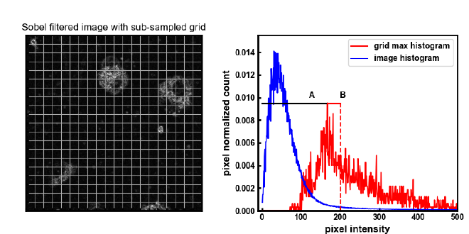
In the plot on the right, the blue line is the histogram of inensity values for the whole image. This histogram shows that the majority of the pixels in the image have a low intensity value or that they are dark background pixels. Pixels that we wish to include in the threshold are those with higher intensities that show up in histograms distribution tail to the right.

This method is based on the idea that the majority of the image area is background and does not contain information that we want to include in the threshold. If we assume that any group of pixels we sample from an image are likely background pixels, then pixels above the maximum value of that subsample are likely to contain information we wish to include in a threshold.

The code to perform image thresholding using the above description is given right here:

import numpy

def thresholdImage(image, offset, coarseness):

    '''
    threshold intinsity image by subsampling the image background
    image:       uint16 mxn array
    offset:      float ratio that threshold value is increased over peak of subsampled max histogram
    coarseness:  int   size of the image subsample grid in n*x*n pixels

    '''
   

    xyDim = image.shape
    max_pix_hist = np.zeros(2**16, dtype = 'uint16')

    # Create row and column vectors to subsample image    
    rc_i = np.array([[r,c] for r in np.arange(start = 0, stop = xyDim[0], step = coarseness) for c in np.arange(start = 0, stop = xyDim[1], step = courseness)], dtype = 'int')
    rc_e = rc_i + coarseness
    for (ri,ci), (re, ce) in zip(rc_i, rc_e):
        
        imseg = image[ri:re, ci:ce]
        max_pix = np.max(imseg)
        max_pix_hist[max_pix] += 1
      
    # Find max value of histogram segments
    k_segment = np.argmax(max_pix_hist[1:])+1
 
    # now that value is a bit off so nudge it up a bit.
    if offset == None:
        thresholdValue = k_segment
    
    else:
        maxind        = 1 
        maxoffset     = abs(k_segment-maxind)+1
        thresholdValue = int(offset*maxoffset+maxind)
     
    return  thresholdValue

The method works by first dividing the image into sub-sections. The size of these sections are given by the variable coarseness which describes a nxn subgrid of an image. The maximum value of each of these subgrids is used as a vote to creat the maximum pixel histogram (max_pix_hist). Next the peak of the maximum pixel histogram (max_pix_hist) is found. The threshold value is then a percentage of the distance (an offseet) after the peak of the maximum pixel histogram given by a ratio of that distance usually 1.1 or 1.2.

This thresholding method seems to be stable and fairly robust when paired with morphological erode and dialate operations that act as a low pass filter. In this way the threshold is set low enough that it still picks up some background but only as single or a few pixels. A combination of dialate and erode operations will then erase the small groups of pixels but preserver the larger blobs of pixels.

I hope someone finds it usefull.

Segment cell nucleus with HOECHST and Draq7 stain

#

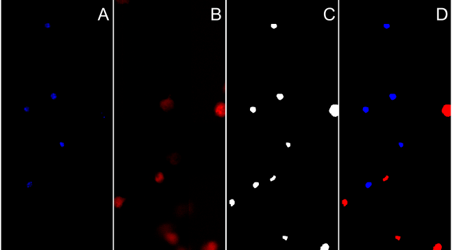
1. take fluorescent image(s)
2. threshold image on nucleus using either the same techniques as above or a set threshold.
3. morphological operations to close cell area

Segment Cell Area

#

Identifying the area a cell ocupies can be difficult but the method described here is a pretty starndard method. It consists of calculating the mangitude of the Sobel gradient. A simple explanation is this method finds regions where neigboring pixels have large intensity differences in the x and y directions. After finding the Sobel gradient magnitude, the resulting image has a threshold calculated followed by morphological and flood fill operations to link and fill the cell area. Overall these steps are depicted in the figure below.

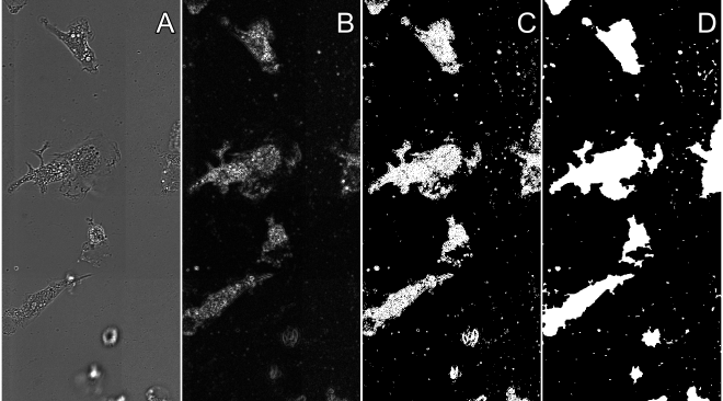
1. Calculate the sobel gradient magnitude of the image using the function below The first step is to use a Sobel filter on the image and get the gradients in x and y. Then just use those values to find the euclidian magnitude of those values. The advantage of calculating the gradient magnitude is that only areas of the image that have high contrast are depected in the resulting image. Variations in the image background are also minimized.

# Dependancies for this function
import cv2
import numpy

def SobelGradient(image):
    '''
    Calculate the Sobel Graident Magnitude of the image 

    input:  uint16 image
    output: uint16 image 
    '''

    # first fine the x and y gradients of the image
    sobelx = cv2.Sobel(image,cv2.CV_64F,1,0,ksize=3)
    sobely = cv2.Sobel(image,cv2.CV_64F,0,1,ksize=3)

    # next find the magnitude of the x and y components
    gradientImage = (sobelx**2+sobely**2)**0.5

    return gradientImage.astype('uint16') 

2. calculate threshold on the sobel gradient magnitude image (see above)

3. morphological operations to close cell area

# Dependancies for this function
import numpy
import cv2

def morphImage(image, thresholdValue, kernel_size)
    '''
    Perform a threshold, morphological, and flood fill operations to segment a image.

    image:          uint16 mxn array that has previously had a threshold calculated
    thresholdValue: uint16 value 
    kernel_size:    uint   value that describes the kernel element size to erode and dialate the image features.
    bwBf0:          uint8 mxn array with morphological operations applied
    '''
    im_dims = image.shape
    ekernel  = cv2.getStructuringElement(cv2.MORPH_ELLIPSE, (kernel_size_, kernelsize))
    bwBf0     = np.greater(image, thresholdValue).astype('uint8')
    
    bwBf0     = cv2.dilate( bwBf0, ekernel, iterations = 2)
    bwBf0     = cv2.erode(  bwBf0, ekernel, iterations = 2)

    _, _, mask, _ = cv2.floodFill(bwBf0.astype('uint8'), None, (0,0), 0)
    bwBf0 = np.array(mask[1:-1,1:-1]==0, dtype = 'uint8')
 
    return bwBf0

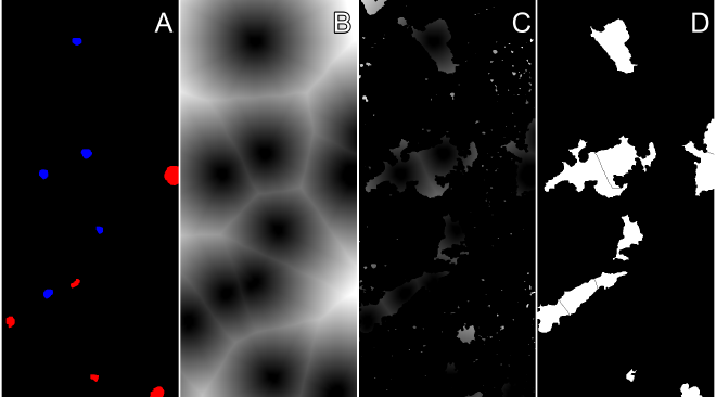
Watershed algorithm to estimate overlaping cell boundaries.

#

4. Perform multiple dialate operations to create gradiant around nucleus

5. Utilize watershed to estimate overlaping cell boundaries

Watershed algorithms are popular for segmenting cells. This method requires having three images that have been thresholded and binariezed, the Draq7 flourescent image, the Hoechst fluorescent image, and the cell area that was found in a previous section. The images in the above figure show the combined Draq7 and Hoecht flourscent signals. Next we label the nucleus areas using the openCV function connectedComponents. This function takes groups of connected pixels and labels them so the group can be indiviually addressed and identified. Following labeling of the nuclei we create a markers image array. The composition of this image array is that cell area we wish to associate with an individual nuclie, the individual pixels are set to zero, pixels that are background are set to one, and the labeled pixels are added into the array. Finally, we need to create a gradient for the watershed to fill. This gradient is nicely done using openCVs distanceTransform function. The function calculates the distance that a particular pixel is from the nearest zero valued pixel. If our starting array is the inverse of the nuclei booleen array (where nuclei pixels are labeled with zeros and all other pixels as ones), the function will return an image where the pixel intensities are the distance from the closest nucleus as shown in (B). We then overlay the distance tranform with the cell area found from the Sobel gradient magnitude. At this point just make sure the markers array is a 32bit signed integer and the gradient image is a 24 or 32 bit RGB image and we can run the watershed.

def segregate_cells(cell_area, draq7_nucleus, Hoechst_nucleus):
    '''
    cell_area:  bool mxn array generated by thresholding the Sobel gradient magnitude
    draq7_nucleus:  bool mxn array generated by thresholding a flourescent image of cells with draq7 dye
    Hoechst_nucleus:  bool mxn array generated by thresholding a flourescent image of cells stained wth Hoechst dye
    '''
    # take binary images of cell nuclei idenfied from fluorescent images
    # Cy5 is the filter set that Draq7 was recorded in and DAPI was the filter set for HEOCHST
    liveandDead = draq7_nucleus | Hoechest_nucleus
    # label the connected component pixels so that individual nuclei can be idenitid
    retval, labels	=	cv2.connectedComponents(liveandDead.astype('uint8'), ltype = cv2.CV_16U)
    # create a marker array where the cell area we wish to associate with a nuclei has zero values and all other areas are 1s
    markers = np.array(~cell_area, dtype = 'int32')
    # then add in the labels of the connected components identified earlier
    markers += labels.astype('int32')
    # next create the gradient by usign the distance transform to calculate how far away a given pixel is from a nucleus
    neg_live = np.array(~liveandDead, dtype  = 'uint8')
    # we invert the booleen image so that the nuclei have values of zero and the distances are calcualted directly.
    nucleus_dist =  cv2.distanceTransform(neg_live, cv2.DIST_L2,5)
    # perform some masking of the cell areas to make sure we limit ourselves to the cell extents
    nucleus_mask =  np.clip(cell_area * nucleus_dist, a_min = 0, a_max = 255).astype('uint8')
    # finally take the watershed but make sure the input image is mxnx3 uint8 and the markers array is mxn int32
    cell_area_labels = cv2.watershed(np.repeat(nucleus_mask[:,:,np.newaxis], 3, axis = 2), markers) 
    # cell areas are anything with a value greater than one.
    segmented_cells= cell_area_labels>1

    # The boundaries of cells will be a value of -1
    segmented_outlines = cell_labels == -1

    return segmented_cells, segmented_outlines

Add layers together

#

6. make final segmented image by adding together individual image segments.

The final step is to take all of the binarized images created during the previous steps and add them together.

def create_training_mask(segmented_cells, segmented_outlines,Hoechst_nucleus, draq7_nucleus):

    image_sit = segmented_cells.shape
    maskImage = np.zeros((image_size), dtype = 'int64')

    maskImage[segmented_cells]    = 1
    maskImage[segmented_outlines] = 2
    maskImage[Hoechst_nucleus]    = 3
    maskImage[draq7_nucleus]      = 4

    return maskImage

Now we have the segmented and classified the images for training the neural network.